Quantization has been adopted by many model providers to reduce inference cost. In my previous LLM system blog, I briefly covered quantization. This article is a more detailed review of modern quantization formats and methods, plus an informal analysis of how quantization is done by leading AI labs.

Quantization formats

There are many design details of a quantization format. The main format is the element precision. Beyond the main format, many factors could also impact the quantization quality of a model. Below is a list of design details of quantization:

• Element precision (Main format): The bit-width and format of quantized values. E2M1 (FP4), E0M3, Int4, E4M3 (FP8 inference), E5M2 (FP8 training), Int8. The ExMy notation indicates x exponent bits and y mantissa bits.

• Scale precision: The precision used for scaling factors, traditionally FP32. Microscaling formats like E4M3, UE8M0 enable better hardware acceleration and can further reduce memory overhead.

• Block format: The number of elements sharing a scale factor. Fine-grained scaling (per-channel, small blocks like 32x1) provides better accuracy by adapting to local distributions, while coarse-grained (per-tensor) is computationally cheaper but less accurate.

• Scale calculation: Dynamic scaling (calculated per step, best accuracy but slower, also called current scaling in training), Static scaling (pre-computed via calibration, inference only), or Delayed scaling (using historical statistics, training only). Dynamic provides better accuracy while static reduces runtime overhead.

• Affine vs symmetric: Symmetric quantization maps data symmetrically around zero (computationally simpler), while affine quantization allows asymmetric mapping with zero-point parameters (better for non-zero-centered data but requires additional storage).

• Quantization targets: Different model components can be quantized - weights (easiest, static), activations (more savings but dynamic ranges), KV cache (addresses memory bottlenecks), attention math, and AllReduce (system-level optimizations).

• Second-level scale: Used in NVFP4 with hierarchical scaling - FP32 second-level scales handle outer range while E4M3 first-level scales manage local precision. This extends representable dynamic range beyond single-level scaling (max value 2688).

A summary of prominent quantization formats and algorithms adopted by frontier LLMs is shown below:

Model & Main Format	Format Details	Quantization Method
Llama 3 & 4 (FP8)	Weights & Activations: 1D-channel FP32 scaling, dynamic scaling	PTQ with online activation clipping
DeepSeek V3 & R1 (FP8)	Weights: 128×128 2D-block FP32 scaling Activations: 128×1 1D-block FP32 scaling, dynamic scaling	Native quantized training
DeepSeek V3.1 (FP8)	Same as DeepSeek V3, except UE8M0 instead of FP32 scaling	Not disclosed; likely native quantized training
GPT-OSS (FP4)	Weights: 32×1 1D-block UE8M0 scaling (MXFP4)	Not disclosed; likely quantization-aware training
Kimi-K2 (FP8)	Same as DeepSeek V3	Post-training quantization
DeepSeek, Kimi-K2, Llama4 (NVIDIA releases, FP4)	Weights & Activations: 16×1 1D-block E4M3 scaling, FP32 second-level scaling (NVFP4)	Post-training quantization

Quantization methods

Post-training quantization (PTQ)

PTQ is a simple and cost-effective method for quantization that requires no modifications to the original training process. The process is sometimes also called calibration, where quantization parameters are determined using a representative dataset. With PTQ, training and inference are completely decoupled, making it attractive for practitioners without access to original training pipelines.

The simplest PTQ method is max calibration, which works surprisingly well in many cases. More sophisticated methods for LLMs include GPTQ and AWQ. These advanced methods achieve better accuracy at most times.

PTQ works quite well for FP8 on almost all LLMs, due to FP8’s sufficient precision. For NVFP4, PTQ also works well for very large models where parameter abundance provides robustness to quantization noise.

Native Quantized Training

Native quantized training traces its origins to mixed precision training (FP16/BF16), as both approaches share the primary goal of reducing the computational cost of training. Pretraining is typically compute-bound, since batch sizes can be made arbitrarily large. While memory savings are also a potential benefit, they are often marginal and depend on the specific implementation.

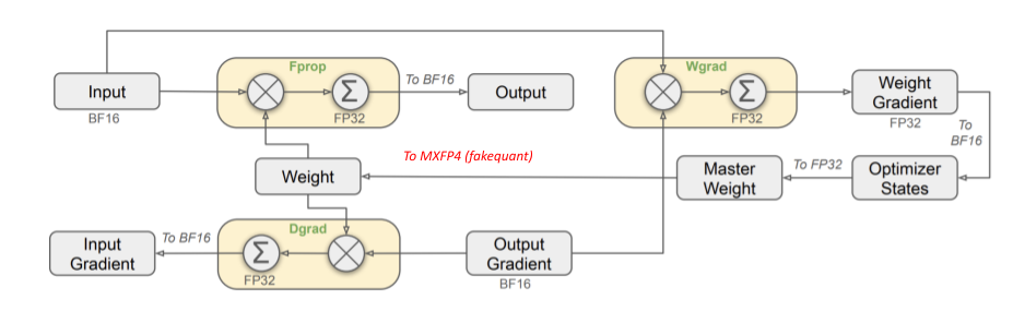
The following illustration, from the DeepSeek V3 tech report, demonstrates FP8 native quantized training. The core idea is to quantize three GEMMs — Fprop, Wgrad, and Dgrad. To perform these GEMMs in low precision, all three of their inputs — Input (activation), Weight, and Output Gradient — must be quantized to FP8.

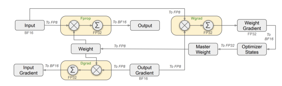
Retaining FP32 master weights is one key idea carried over from mixed precision training to native quantized training. This design is fundamental for effective convergence. Several works have further optimized FP8 training, including:

• Fine-grained block scaling, such as DeepSeek’s 2D block scaling, which offers better numerical stability than tensor-level scaling.
• Optimizer state quantization, which provides significant memory savings; see Microsoft FP8-LM.

FP4 pretraining advances compute efficiency even further beyond FP8, but the more aggressive nature of FP4 quantization necessitates additional optimizations. The most crucial techniques are Random Hadamard Transformation (RHT) and stochastic rounding (SR), both of which help to smooth the gradient distribution and mitigate quantization error. These methods have been adopted in several notable works, including those from Amazon, ISTA, and most recently NVIDIA.

Compared to PTQ, native quantized training is a significantly more ambitious undertaking, both technically and organizationally. Technically, training must be sensitive enough to capture subtle weight updates to ensure effective learning under quantization constraints. Organizationally, the training team bears responsibility for both model accuracy and the development of new models. Quantized training can introduce additional uncertainty into this process—for example, whether a problem is due to model design or quantization. In contrast, quantization for inference is more closely aligned with the inference team’s focus on cost reduction.

Quantization Aware Training (QAT)

What sets QAT apart from native quantized training?

• Purpose-wise, QAT targets inference speedup and accuracy recovery, while quantized training targets training speedup.

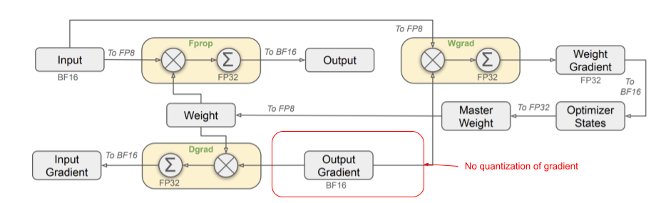
• Implementation-wise, the key distinction is that QAT only focuses on forward pass and does not quantize gradients. In addition, QAT typically involves a brief period of additional training on top of a trained model.

QAT is specifically designed to recover accuracy for the inference stage, so there is no need to quantize gradients. With gradients remaining in full precision, the two backward GEMMs—Wgrad and Dgrad—are computed in high precision rather than low precision. As in native quantized training, FP32 master weights are maintained to ensure stable convergence.

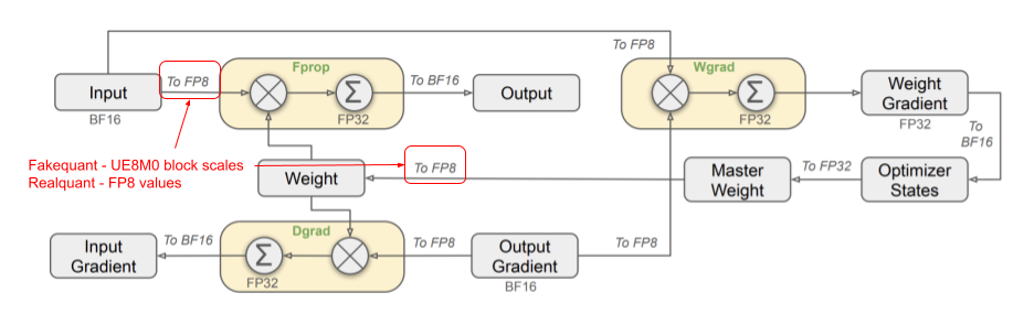
Fakequant is a common feature in QAT, though it is not strictly tied with QAT. In reality, QAT can also employ real quantization. Fakequant refers to representing and computing low-precision values using high-precision formats—for example, storing int8 values in fp32. This approach sacrifices speed for compatibility, allowing the same kernels to be used across different GPUs and enabling low-precision emulation regardless of hardware support (see the table below).

GPU generation	Native precisions
Volta, Turing	Int4, Int8, FP16
Ampere	Int4, Int8, BF16, FP16
Hopper, Ada Lovelace	Int8, FP8, BF16, FP16
Blackwell	MXFP4, NVFP4, Int8, FP8, MXFP8, etc

QAT optimizations primarily focus on training data, loss functions, and the design of quantized forward and backward passes, as QAT is less constrained by training speed. Some optimizations, such as stochastic rounding, are shared between QAT and native quantized training. Notable QAT methods include LSQ, QKD, and Data-free LLM-QAT.

While QAT sits at the intersection of training and inference teams, it is generally easier to manage uncertainty, define boundaries, and allocate responsibilities compared to native quantized training. From my experience, QAT has been widely adopted in leading AI labs for both cost savings and accuracy preservation.

DeepSeek V3.1 and GPT-OSS Discussion

With the conceptual framework established above, we can now analyze the quantization approaches used in DeepSeek V3.1 and GPT-OSS.

DeepSeek V3.1 FP8 with UE8M0 scaling: Assuming DeepSeek did not have access to Blackwell GPUs, DeepSeek V3.1 was trained using native FP8 quantized training, supplemented by fakequant UE8M0 scaling factors. Again, fakequant is not exclusive to QAT. Since gradients are quantized, this approach should still be classified as native quantized training.

During FP8 quantization of weights and activations, UE8M0 scaling factors can be generated and stored as FP32 values. Because these scaling factors are small, this fakequant step should be extremely fast and do not impact training speed. The overall training pipeline closely resembles that of V3/R1, while at inference time, the model can take advantage of hardware with native MXFP8 support, such as Blackwell.

GPT-OSS weight-only MXFP4: Although OpenAI has not disclosed their MXFP4 quantization recipe, the fact that model activations are not quantized suggests that gradients quantization would be unnecessary. Therefore, GPT-OSS was likely quantized using QAT rather than native MXFP4 training. Moreover, native MXFP4 training would require large deployment of Blackwell GPUs, which was not quite feasible within the release timeframe of GPT-OSS.