Understanding LLM System with 3-layer Abstraction
Performance optimization of LLM systems requires a thorough understanding of the full software stack. Somehow I couldn’t find a comprehensive article that covers the big picture yet, so instead of waiting for one, I decided to write this article. This article is not a comprehensive review or best practice guide, but rather a sharing of my overall perspective on the current LLM system landscape.
First, any system is designed to achieve specific objectives within given constraints. For LLM systems, the most critical objectives are throughput and latency. These two objectives must be optimized within three fundamental constraints: compute (hardware operation speed and supported types), memory (capacity and hierarchy), and communication (memory & network bandwidth, latency, and hierarchy). Google provides excellent coverage of these concepts in the Roofline section of their Scaling Book.
Explain 3-layer Abstraction
To navigate the complexity of modern LLM systems, I find it helpful to think in terms of three distinct abstraction layers. Each layer addresses different types of constraints and optimization opportunities, creating a good framework for understanding and improvement, which we will cover in details.
The table below summarizes the basics of 3 abstraction layers.
| Abstraction Layer | Operations | Representative Software |
|---|---|---|
| Kernel | Scalar/Vector/Tile instructions | CUDA C/C++ & PTX, Triton |
| Graph | Tensor primitives | PyTorch, JAX, TensorRT, ONNXRuntime |
| System | Sharding, Batching, Offloading, .. | TensorRT-LLM, vLLM, Megatron-LM, VeRL |
It should be noted that Triton and CUDA belong in the same category, despite Triton’s higher-level interface, both fundamentally optimize performance at the compiler and micro-architecture level. Similarly, while PyTorch and TensorRT serve different use cases, they both operate on tensor-level abstractions and optimize the model graph as a whole.
Let’s examine each layer in detail, starting from the lowest level of abstraction.
Kernel layer
The kernel layer focuses on software execution at the micro-architecture level. A kernel is the smallest unit of workload executed on an accelerator, including GPU.
The programming model at this layer maps available hardware resources (general-purpose cores, matrix multiplication units, near-processor memory, GPU memory) to programming concepts (threads & blocks, local memory, global memory) and exposes the necessary instructions for users to manipulate them.
CUDA C/C++ language has been the de facto standard for GPU kernel programming. As the need of kernel programming increases in recent years, a number of choices at this layer have become available. Two different trends are observed, which are not mutually exclusive:
-
Tile languages like Triton, CuTile, and TileLang elevate the control granularity from thread to block and data granularity from scalar to tile. Users only handle block-level logic while intra-block arrangement is delegated to the compiler. This approach offers two key advantages: simpler programming for users, especially machine learning engineers and researchers; and easier maintenance of cross-platform compatibility. For example, whether to use 128x32 MMA instructions or 32x32 MMA instructions is now decided by the compiler rather than users, making it easier to support different hardware.
-
Template frameworks like CUTLASS. Since matrix multiplication is the most important optimization problem in kernel programming, CUTLASS handles the core matrix multiplication while leaving customizable “peripheral” code to users, but users still have full control of the code.
Kernel performance is measured by latency (throughput is also mapped to latency of different input shapes). Most optimization techniques can be categorized into:
- Data locality. Example: utilize near-processor register, cache and shared memory to avoid data movement.
- Data movement efficiency. Example: use swizzling to avoid bank conflicts; overlap data loading and computation.
- Special instructions. Example: use TensorCore MMA (matrix multiplication accumulation) and Hopper TMA (tensor memory accelerator).
There are also specific optimizations for different hardware or different generations of hardware. Most of them, including NVIDIA GPU, do not have detailed public documentation on the low-level details.
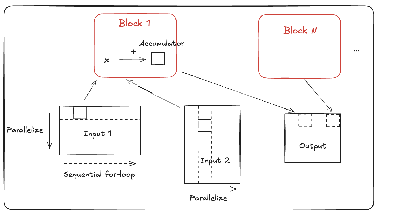
Several key points to note:
- For output data locality, this kernel uses output tiling, i.e., splitting the workload by output tiles, and distributes partitioned workloads, i.e., blocks to each processor. In this way the accumulator can be held locally, avoiding read/write to main memory.
- For input data locality, because each block reads a row of tiles from input 1 and a column of tiles from input 2, it leverages L2 cache by launching blocks in “grouped ordering” to reuse input data.
- Within a block, the arithemic operations are described in tile language, and Triton compiles the tile language to hardware instructions. This differs from CUDA, where users have fine-grained control along with the responsibility to low-level CUDA cores, TensorCore, and shared memory.
Underlying the programming tile, the actual MMA size depends on the hardware. For example, H100 GPU supports 256x64x16 FP16 MMA, and TPU (prior to v6e) supports 8x128x128 BF16 MMA.
Another excellent example is online softmax in Flash Attention. Softmax is normally computed on a full row of the attention matrix, which requires substantial data movement. Online softmax solves this problem by converting the global formula to a recurrent formula. In this new recurrent formulation, no reads or writes from global memory are required.
Graph layer
The graph layer focuses on optimizing the model graph executed on a single GPU. Programming at this layer emphasizes composability and ease of modification. Historically, composability came at the cost of performance, which is why ONNXRuntime, TensorRT, FasterTransformer were used for serious infence scenarios. Today, PyTorch has gradually overcome its original weakness and captured significant inference market, attributing to two factors: reduced overhead from CUDA Graphs, torch.compile, etc; increased model workload like LLM that dwarf framework overheads.
Graph-level optimizations exploit the characteristics of consecutive kernels and the inherent properties of ML models. The overarching goal remains reducing communication and memory usage while improving compute efficiency. Specifically, there are the following common types of optimization:
Merging converts multiple tensor operations into a single mathematically equivalent operation. Examples include Conv/BatchNorm merging and Multi-FC merging. A recent merging technique is MLA weight absorb which enables decode-time memory saving at the cost of more computation.
Fusion is another commonly used technique and often confuses with merging. It combines multiple kernels without altering the mathematical formulation. This technique overlaps communication with computation, avoids writeback to main memory, and reduces kernel launch overhead. For example, Conv/ReLU fusion performs in-place ReLU operations instead of writing/reading to the main memory. In multi-GPU inference, GEMM/AllReduce fusion is sometimes to reduce latency, which synchronizes partial outputs immediately upon computation.
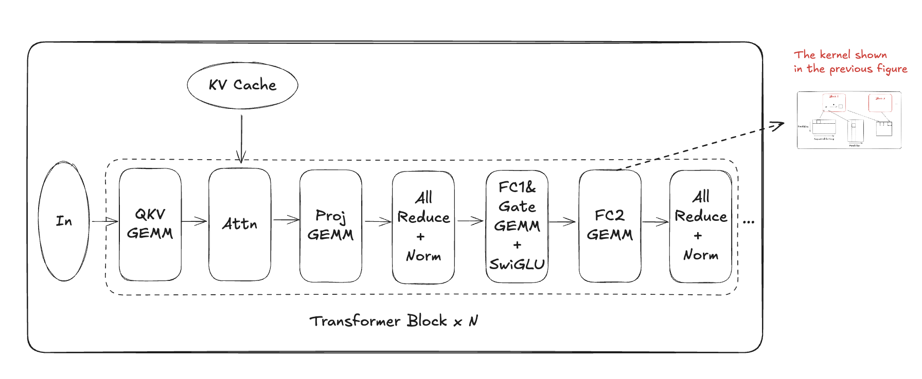
Merging is denoted by & and fusion is denoted by +.
Quantization aka low precision, is one of the most widely used techniques in ML system optimization and a great example of algorithm/hardware co-evolution. In the CNN era, 8-bit quantization is typically good enough. In the LLM era, the need for more compression keeps pushing the frontier of quantization. I initialized and have been working on TensorRT Model Optimizer for the past few years and we have a brief description of quantization. Some general observations on the current stage of quantization:
- Quantization extends beyond most common weight quantization to activations, KV cache, gradients, and communication.
- Inference typically leads training in precision reduction. As of 2025, FP4 is largely de-risked for inference with FP8 already becoming mainstream, while training shows early FP8 adoption with BF16 as the standard.
Sparsity has deep historical roots, tracing back to Yann LeCun’s Optimal Brain Damage (1989), and was revitalized for modern neural networks through works like Deep Compression. Early research concentrated on static sparsity approaches, including fine-grained weight pruning, channel pruning, and 2:4 sparsity patterns. In the LLM era, evidence suggests total parameter count significantly impacts performance, driving increased interest in dynamic sparsity techniques such as prefill sparsity, compressed KV cache and dynamic KV loading.
Additional common GPU optimizations include CUDA graphs and multi-stream execution. CUDA graphs pre-record kernel dependency graphs to reduce launch latency, while multi-stream execution overlaps small-workload kernels to improve GPU utilization.
More graph-level optimizations actually occur during model design within hardware constraints, as the Hardware Lottery suggests. Early examples include Group Convolution, designed to reduce convolution’s computational density. In the LLM era, bandwidth constraints drive architectural innovations like Mixture of Experts (MoE), Grouped Query Attention (GQA), Multi-Head Latent Attention (MLA), and State Space Models (SSM). MoE can be conceptualized as trained dynamic sparsity, with notable similarities to hard attention mechanisms when viewing expert weights as activated tokens.
System layer
This layer deals with the resources needed by a model and the constraints of a pod - the minimum repeatable deployment unit. As an example, DeepSeek V3 has an official implementation with inference pods of 176 GPUs and a training pod (whole cluster) of 2048 GPUs. At the system level, we pay less attention to the internal details of a model, but abstract it as an elastic program (engine) with computation, memory, and communication need.
Starting from this layer, inference and training frameworks diverge significantly. Inference frameworks like vLLM, SGLang, and TensorRT-LLM emphasize high-performance kernel, parallelism, smart request batching, and efficient KV management. Training frameworks iterate rapidly as algorithms evolve, with many serving as scaffolds for parallelism implementation (e.g., Megatron-LM, DeepSpeed). With the recent rise of Reinforcement Learning, there are more connections between training and inference - for example, VeRL emphasizes seamless integration of Megatron-LM, vLLM, and other frameworks.
Again, we focus on optimizations that better utilize system computation, memory, and communication.
Parallelism is the key for both training and inference. There are many good explanations available, e.g., NeMo Documentation and DeepSpeed Documentation.
Almost all parallelism strategies improve throughput. Not all of them improve latency. Choices of parallelism is determined by memory and communication constraints. Overall computation is mostly a constant except for corner cases like FSDP and TP vs DP Attention. Below is a table summarizing most common parallelism strategies.
| Type | Description | Pros & Cons |
|---|---|---|
| Data parallel | Parallelize at batch dimension | No improvement for latency. No communication during inference and low communication during training. |
| Pipeline parallel | Parallelize at batch and layer dimensions | No improvement for latency. Low communication for both inference and training. Saves model memory. |
| Tensor parallel | Parallelize FC layers at row&column dimensions and attention at head dimension | Improves latency. High communication cost. Saves model memory. |
| Expert parallel | Parallelize MoE at expert dimension | Improves latency at large-batch regions. Lower communication cost than TP when activated experts are fewer than TP ranks. Saves model memory. |
| Sequence parallel | Parallelize layernorm or attention projection layers at sequence dimension | Augments tensor parallel. Low communication cost. |
| Context parallel | Parallelize all layers at sequence dimension | Improves latency for long context prefill. High communication cost. |
| ZeRO | Shard optimizer states (stage 1), gradients (stage 2), and weights (stage 3) | Mainly for training. Overlaps computation and communication, but each shard still carries full computation. |
| FSDP | Shard weights, gradients and optimizer states | Almost identical to ZeRO, see the mapping between FSDP & DeepSpeed. |
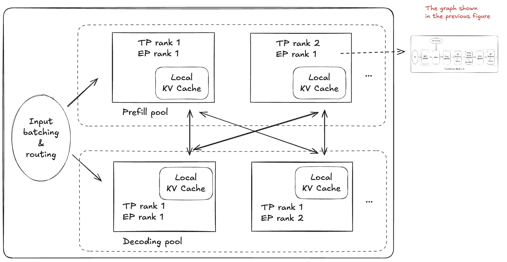
To choose the right parallelism for inference, when the model size is not too large (<100GB), a common practice is to scale up tensor parallelism to the point where communication latency becomes non-trivial, then scale out with pipeline parallelism and data parallelism. For highly sparse MoE models, TP may not be favored over EP and choosing the right parallelism in a cluster becomes more difficult. This is why we’re seeing tools like NVIDIA Dynamo to optimize parallelism strategies. The complexity also applies to training-time parallelism, which is usually designed and hand-tuned specifically for model architecture and datacenter configurations.
Inference system optimizations
For inference systems, the primary throughput metric is total tokens per second (TPS), while latency metrics are time per output token (TPOT) and time to first token (TTFT).
A no-brainer optimization is to avoid recomputation, with methods like KV cache, prefix caching, offloading, etc. Beyond that, the key of throughput optimization is batching, and many methods are just smart ways of batching. Continuous batching aggregates requests with varying lengths across prefill and decode phases. KV cache optimizations, such as paged attention, expand the maximum feasible batch size within memory constraints. Even latency optimization techniques like speculative decoding can be viewed as forms of batching.
Latency is fundamentally a trade-off with throughput, mediated by parallelism choices. Generally, to reduce per-token generation time, one must necessarily reduce the number of tokens generated concurrently. This relationship was illustrated in a trade-off curve presented at GTC 2025. Somehow, quite a few friends complained to me this figure is counterintuitive.
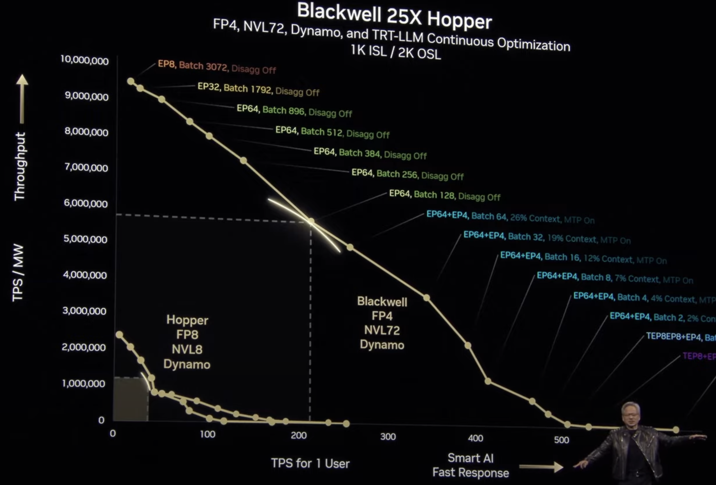
Advanced optimizations that push beyond this trade-off curve include PD disaggregation and speculative decoding. PD disaggregation has been deployed by production LLM serving systems for some time and is now gaining broader ecosystem support through frameworks like SGLang and TensorRT-LLM. Speculative decoding exemplifies algorithm-system co-design and merits detailed discussion in subsequent sections.
Training system optimizations
Compared to inference systems, training systems face different constraints: throughput driven, less stringent latency requirements, but facing rapidly evolving methodologies and model architectures. It often goes through rapid iterations when new architectures or new training techniques are introduced. I personally observed that training systems are less deeply optimized than inference (I don’t take responsibility for this statement. There are exceptions like DeepSeek).
Pretraining used to be the primary focus (probably still is). Operating at massive GPU scales in a throughput-oriented manner, Model FLOPs Utilization (MFU) serves as the key performance metric. Parallelism is the key of optimization, which we has already discussed.
At the scale of pretraining, system resilience becomes critical for maintaining high MFU beyond parallelism strategies. Key techniques include fault tolerance mechanisms and asynchronous checkpointing—see NVIDIA Resiliency Extension for common solutions.
Post-training optimization was historically considered less critical due to its smaller computational scale. However, the rise of Reinforcement Learning (RL) has fundamentally changed this landscape. RL introduces new system-level challenges that extend far beyond traditional parallelism concerns. I call it the parallelism and placement problem, extensively discussed in HybridFlow:
-
Multi-model dependency: The interdependencies between multiple models (actor, critic, reward model, etc.) create a fundamental dilemma—either colocate models at the cost of precious GPU memory, or distribute them across separate GPUs at the cost of compute idle time.
-
Workload heterogeneity: Training and rollout (generation) represent fundamentally different computational patterns. Optimal performance often requires dedicated inference frameworks with periodic weight resharding between iterations.
Reinforcement Learning from Verified Rewards (RLVR) introduces additional complexity. GPU clusters optimized for pretraining typically feature high network bandwidth but relatively modest CPU capabilities. When external reward signals require CPU execution, this can create unexpected bottlenecks in the training pipeline.
While RL system design encompasses both training and inference frameworks, it remains fundamentally a resource allocation problem within datacenter constraints, thus fitting within our system layer abstraction. Looking forward, it will be fascinating to observe whether companies like OpenAI or robotics firms successfully bridge the training loop with external environments—the Internet, simulation worlds, or physical reality.
Exceptions to the 3-Layer Abstraction
While the 3-layer abstraction provides a useful framework for understanding most LLM systems, certain architectures and techniques transcend these boundaries.
Dataflow Architectures and Megakernels. Some ASICs (e.g., SambaNova, Cerebras, Groq) employ data-centric programming models that execute operations immediately when partial data becomes available. In these programming models, a “kernel” can encompass an entire transformer block or even the complete model (see SambaNova’s HotChips 2024 presentation). This design provides significant latency advantages at the cost of programming complexity. The use of high-bandwidth on-chip SRAM is a different topic which is worth another article. Recent GPU community has explored similar concepts, such as MegaKernel, which aims to eliminate GPU idle timethrough massive kernel fusion.
Speculative decoding. Speculative decoding is an elegant technique that stems from system insights (i.e., batching being faster than sequential execution), and is well-engineered with both ML (draft model/head) and statistics (reject sampling) to perfectly match the original model distribution. It shows the power of cross-stack optimization and it is hard to classify it into any single optimization layer. I have no doubt that if transformer continues to prevail in the next ten years, speculative decoding will be a cornerstone just like speculative execution is for modern CPUs.
Final words
System design operates on shifting foundations, where the optimal trade-off between physical constraints, model architecture, and applications continuously evolves. Today’s optimal solutions may become tomorrow’s bottlenecks. Prior to the LLM era, a 2-layer abstraction (kernel and graph layers) sufficiently captured most ML workloads. Nowadays, with the emergence of new training paradigms and application ecosystems, we may soon the need for additional software layers beyond the 3-layer framework presented here.
Acknowledgement: This blog has been revised based on feedbacks from Julien Demouth, Song Han and June Yang.
Additional References
- Semi-analysis: The Memory Wall: https://semianalysis.com/2024/09/03/the-memory-wall/
- Thunderkitten: 2D tile, 1d vector: https://hazyresearch.stanford.edu/blog/2024-05-12-tk
- CUDA talk at GTC 2025: https://www.nvidia.com/en-us/on-demand/session/gtc25-s72383/
- Scaling book: https://jax-ml.github.io/scaling-book/